
Model Predictive Control of a Series Elastic Actuator
Recently I had the pleasure to work on what is probably the best-made Series Elastic Actuator (SEA) module in the world: the ANYdrive. from Robotic Systems Lab at ETH Zürich. I implemented Model Predictive Controller (MPC) for this SEA, but not a normal MPC. No specs or details about the design of the ANYdrive will be discussed since those are proprietary. But feel free take a look at ANYbotics.
The content of this post is extracted from the project report of my research project at ETH Zürich. The full work can be found here
You can click on the blue buttons to navigate in this post.
Introduction Modeling The Controller Experimental Results Conclusion
Introduction
SEA is a special class of actuators that is considered particularly suitable for robots that physically interact with uncertain environments. It consists of a motor and a gearbox, but the load is connected to the output of the gearbox via a spring. This spring acts as a buffer between the environment and the rather stiff gearbox, making the robot compliant (less likely to harm people). The spring also let you sense torque easily, using Hooke’s Law.
The ANYdrive is just an example of such actuators. It is drive by a 3-phase brushless Permanent Magnet Synchronous Motor (PMSM). Instead of using a cascaded loop to control the PMSM, the PMSM AND the spring in series are controlled by a single unified controller. Providing an output torque setpoint, the MPC computes directly the voltage to be applied to the PMSM. This novel MPC is referred to as the Model Based Unified Torque Controller (MBUTC).
Modeling
The first step is to model the ANYdrive. The model contains 2 parts. The first part is the electrical dynamics of the PMSM, and the second part the the dynamics of the mechanical system.
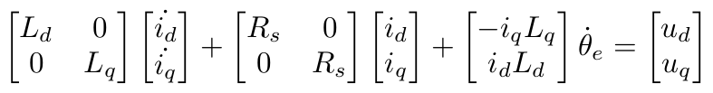
The modeling of the PMSM is well established, and exists in a lot of literatures. Here, the PMSM is modeled using space vector. All 3-phase quantities, currents and voltages, and represented in the DQ coordinate system, which is attached to and rotates with the rotor of the PMSM. The Park Transformation is used to do this job.
In DQ coordinate system the dynamics is greatly simplified, and can be writen down as follows:
The mechanical system is essentially a spring-mass-damper system, and its free-body diagram is shown below:
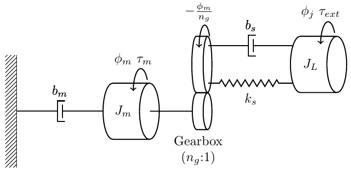
The equation of motion is given by:
\[\begin{equation} J_m\ddot{\phi}_m+(b_m+\frac{b_s}{n_g^2 \eta})\dot{\phi}_m+\frac{k_s}{n_g^2 \eta}\phi_m + f(\dot{\phi}_m) - \frac{k_s}{n_g \eta}\phi_j - \frac{b_s}{n_g \eta}\dot{\phi}_j = \tau_m \end{equation}\] \[\begin{equation} f(\dot{\phi}_m) = F_s\tanh(\frac{2.09}{\omega_{bk}}\dot{\phi}_m) \end{equation}\]For detailed derivations and the meaning of the symbols, please refer to the full work (link to the PDF is given at the beginning of the post).
The nonlinear friction effect is rather strong in this case, and has to be accounted for in the model. Here, the nonlinear friction is modeled as a hyperbolic tangent function of the motor’s velocity. This function is continuous and differentiable w.r.t velocity, which is a very desirable property. In the equation below, Fs is the maximum static friction.
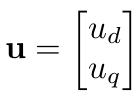
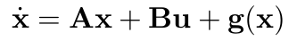
Now we define the state vector, x, and state space matrices, as follows:
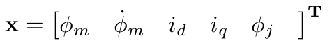
The resulting state space equation of the ANYdrive then looks like this:
In fact all SEAs that are driven by a PMSM can be modeled this way. This model is therefore potentially applicable to many other SEAs.
The parameters of the model are identified in a series of experiments. Then, the response of the real SEA in an experiment is compared to the result of a numerical simulation using the model (implemented in Simulink). Results are seen in figures below.
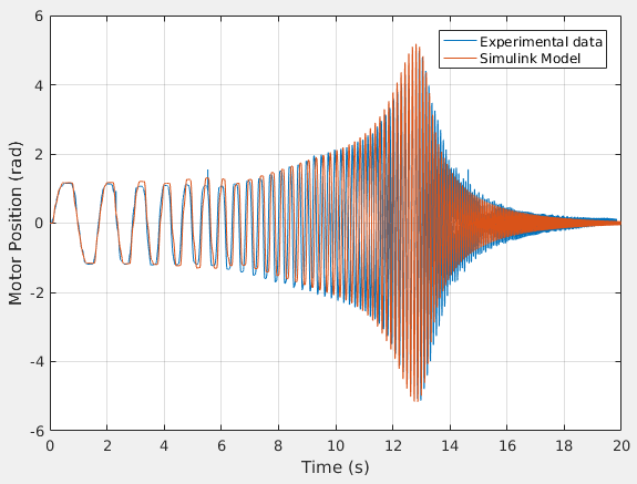
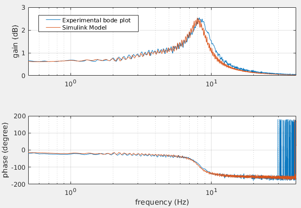
The fact that simulation matches well with experimental data shows the accuracy of the model.
The Controller
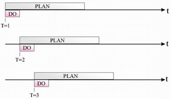
The controller is essentially an MPC that controls the deflection of the spring. The MPC is a form of receding horizon controller. At time step k, the controller computes optimal actions for time steps k+1 ~ k+N (N is called the horizon). However, only the action at k+1 is applied to the system, while actions k+2 ~ k+N are discarded. At time step k+1, the above-mentioned step is repeated. The idea is shown in figure below:
The following steps are involved at each timestep:
- measurements of the state variables are taken.
- desired joint torque is converted to the desired spring deflection (using Hooke’s law).
- the system model derived before is linearized about the measured states.
- formulate a finite-horizon linear-quadratic-regulator (LQR) for the linearized system.
- solve this LOR deterministically, using the dynamic programming algorithm.
- apply the computed optimal action (i.e. voltage) to the motor.
Similar to most MPCs, this control law is relatively computationally expensive. It was a challenge to implement it in the MCU that controls the SEA, which is strictly real-time. The algorithm is optimally divided into a number of stages which run during different hardware interrupt cycles, so the algorithm is able to run deterministically at the desirable frequency.
Experimental Results
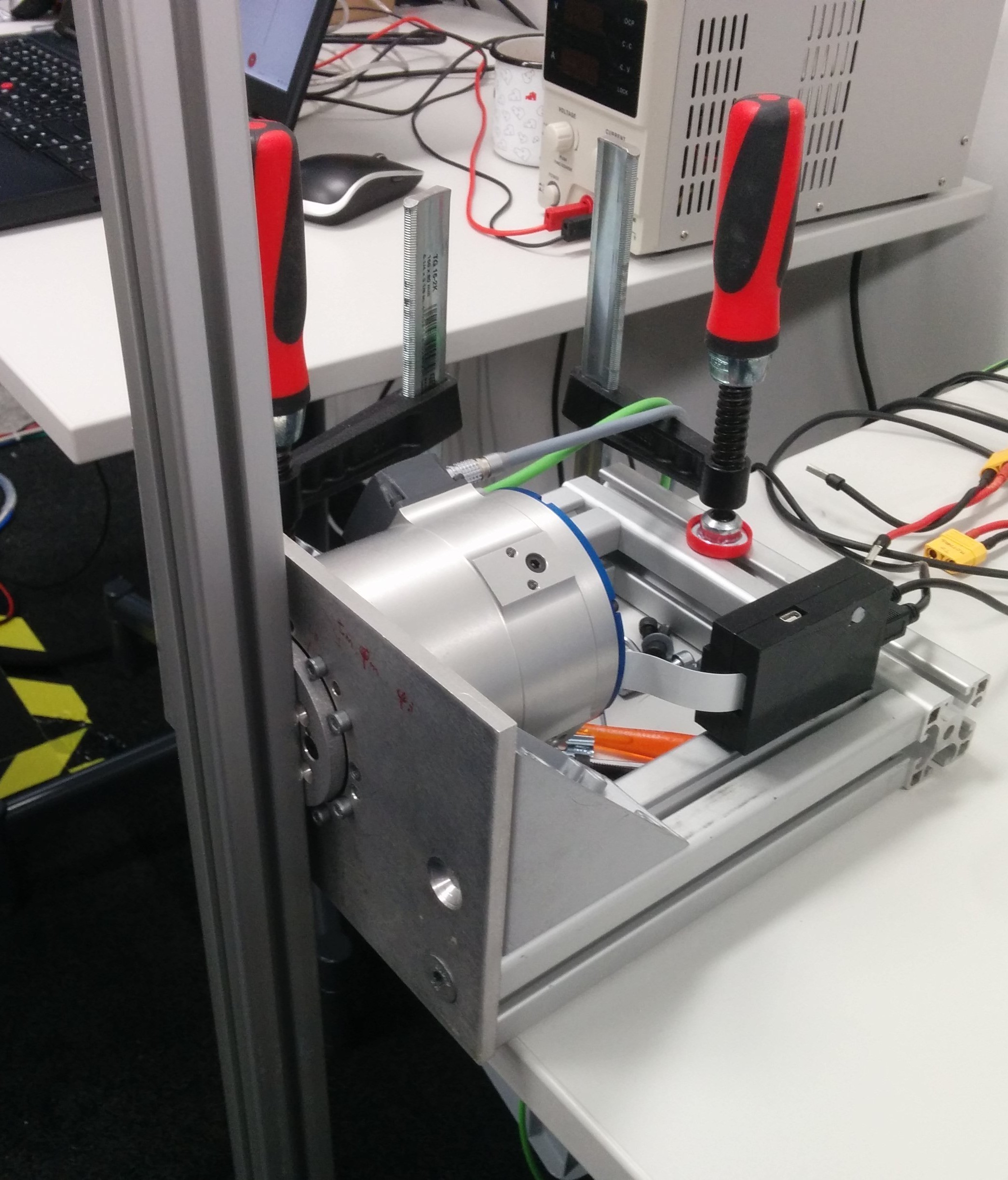
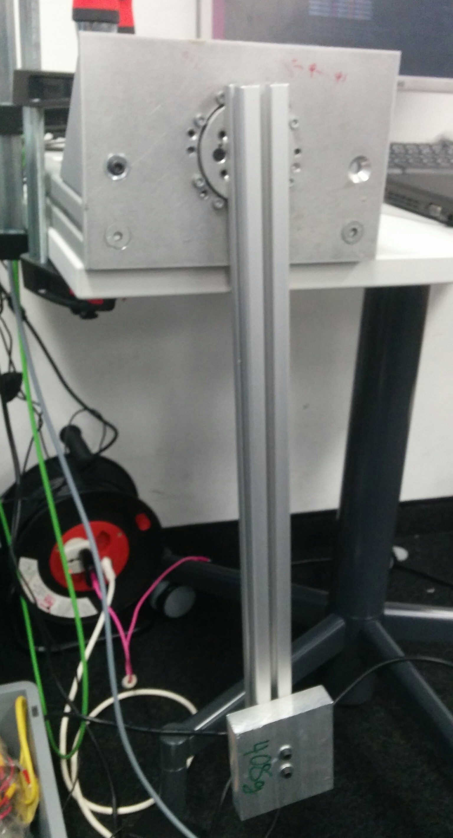
The MBUTC is tested in two different setups. First, the output shaft of the SEA is blocked, so the motor sees an infinite output impedance. Second, a pendulum of an inertia of approximately 0.1 kg m^2 is attached to the output shaft, simulating a more realistic loading condition. The setups are shown in figure below:
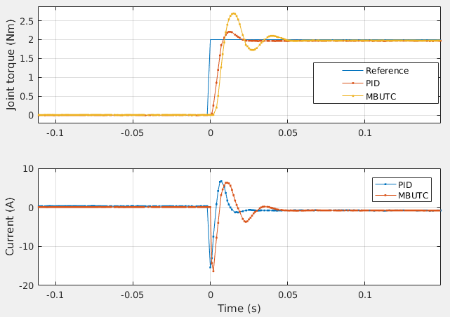
The step response of the MBUTC is measured. The response with the shaft blocked is shown as follow:
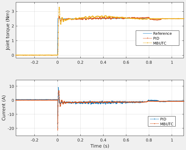
The response with a pendulum attached is shown as follows:
Conclusion
The modeling and system identification of the SEA are satisfactory. However, the MBUTC performs worse than the traditional PID controller with cascaded loops.
A number of possible explanations of the sub-optimal performance:
- the MBUTC does not have a integrator action to eliminate steady-state error.
- the MBUTC is too short-sighted, due to the finite (and short) horizon used here.
- the model of static friction is not perfect (the model is continuous w.r.t velocity, but the real static friction is not).
The most promising candidate for improvement is to add an disturbance observer to this MPC. An disturbance observer will help eliminating steady-state error, and may be able to mitigate the effect of imperfect friction model.
Leave a Comment